Basis use of levelplot()

The lattice package allows to build heatmaps thanks to the levelplot() function.

Input data: here input is a data frame with 3 columns prividing the X and Y coordinate of the cell and its value. (Long format).

# Load the lattice package
library("lattice")
 
# Dummy data
x <- seq(1,10, length.out=20)
y <- seq(1,10, length.out=20)
data <- expand.grid(X=x, Y=y)
data$Z <- runif(400, 0, 5)

## Try it out
levelplot(Z ~ X*Y, data=data  ,xlab="X",
          main="")

From wide input matrix

Previous example of this document was based on a data frame at the long format. Here, a square matrix is used instead. It is the second format understood by the levelplot() function.

Note: here row and column order isn’t respected in the heatmap.

# Load the library
library("lattice")
 
# Dummy data
data <- matrix(runif(100, 0, 5) , 10 , 10)
colnames(data) <- letters[c(1:10)]
rownames(data) <- paste( rep("row",10) , c(1:10) , sep=" ")
 
# plot it flipping the axis
levelplot(data)

Flip and reorder axis

The t() function of R allows to transpose the input matrix, and thus to flip X and Y coordinates.

Moreover, you can reverse matrix order as shown below to reverse order in the heatmap as well. Now the heatmap is organized exactly as the input matrix.

# Load the library
library("lattice")
 
# Dummy data
data <- matrix(runif(100, 0, 5) , 10 , 10)
colnames(data) <- letters[c(1:10)]
rownames(data) <- paste( rep("row",10) , c(1:10) , sep=" ")
 
# plot it flipping the axis
levelplot( t(data[c(nrow(data):1) , ]),
           col.regions=heat.colors(100))

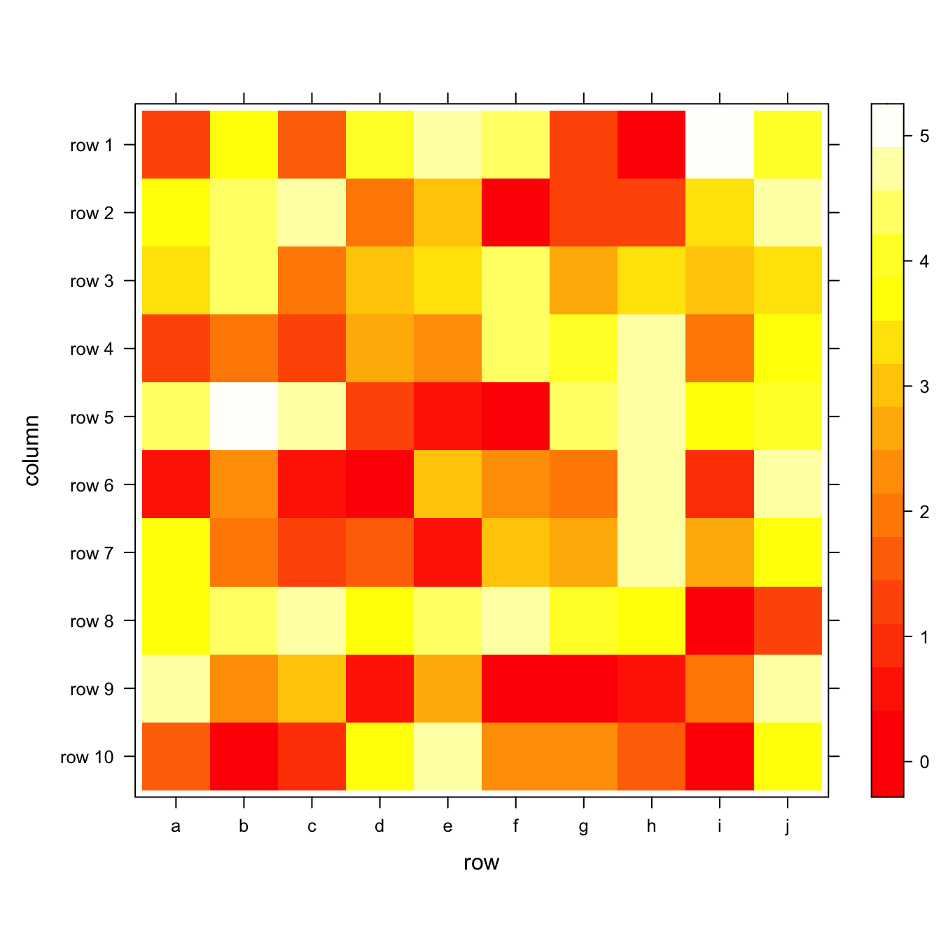
Custom colors

There are several ways to custom the color palette:

native palettes of R: terrain.color(), rainbow(), heat.colors(), topo.colors() or cm.colors()
palettes of RColorBrewer. See list of available palettes here.
palettes of Viridis: viridis, magma, inferno, plasma.

# Lattice package
require(lattice)

# The volcano dataset is provided, it looks like that:
#head(volcano)

# 1: native palette from R
levelplot(volcano, col.regions = terrain.colors(100)) # try cm.colors() or terrain.colors()

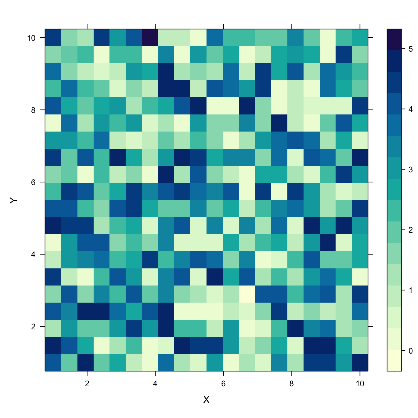
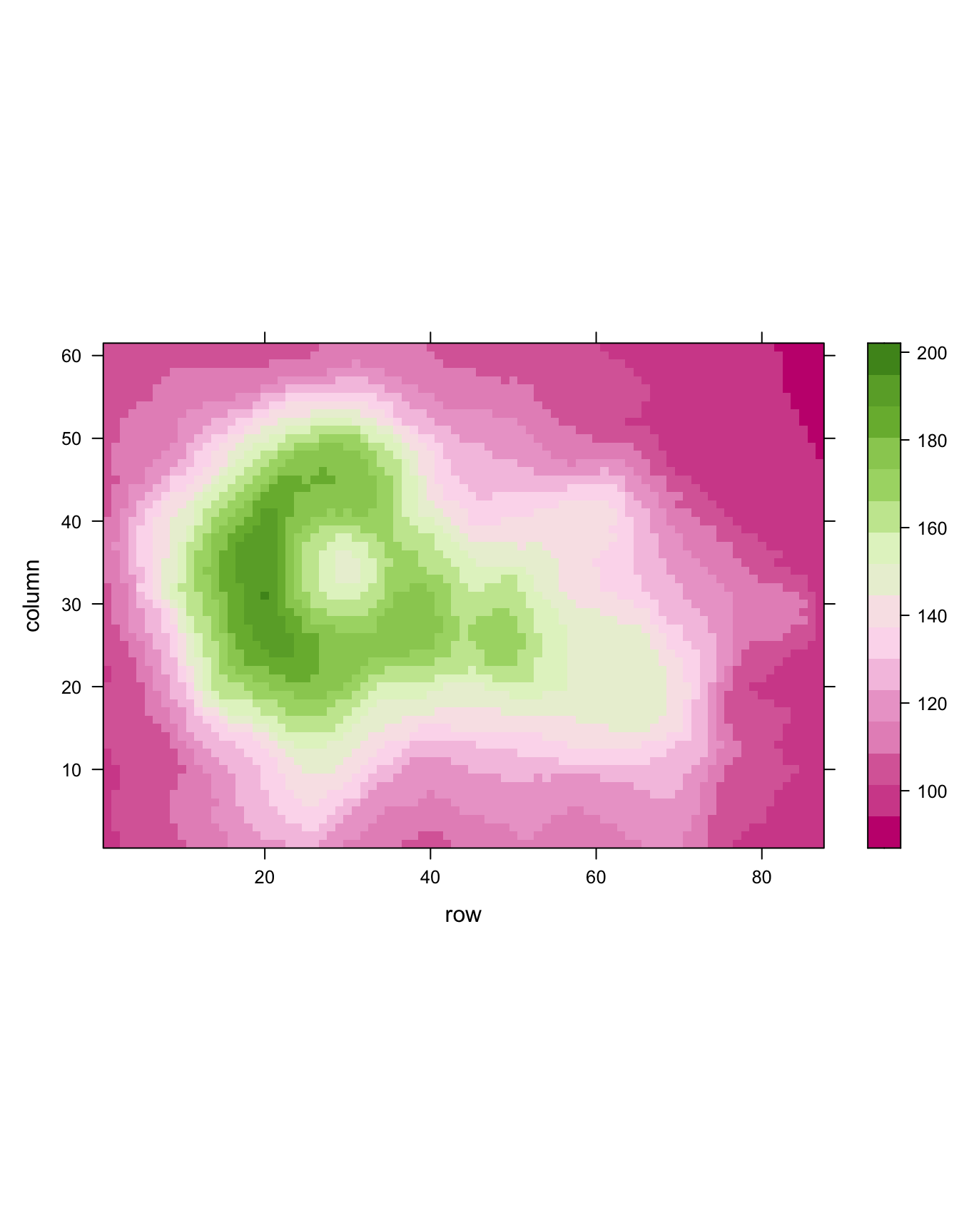
# 2: Rcolorbrewer palette
library(RColorBrewer)
coul <- colorRampPalette(brewer.pal(8, "PiYG"))(25)
levelplot(volcano, col.regions = coul) # try cm.colors() or terrain.colors()

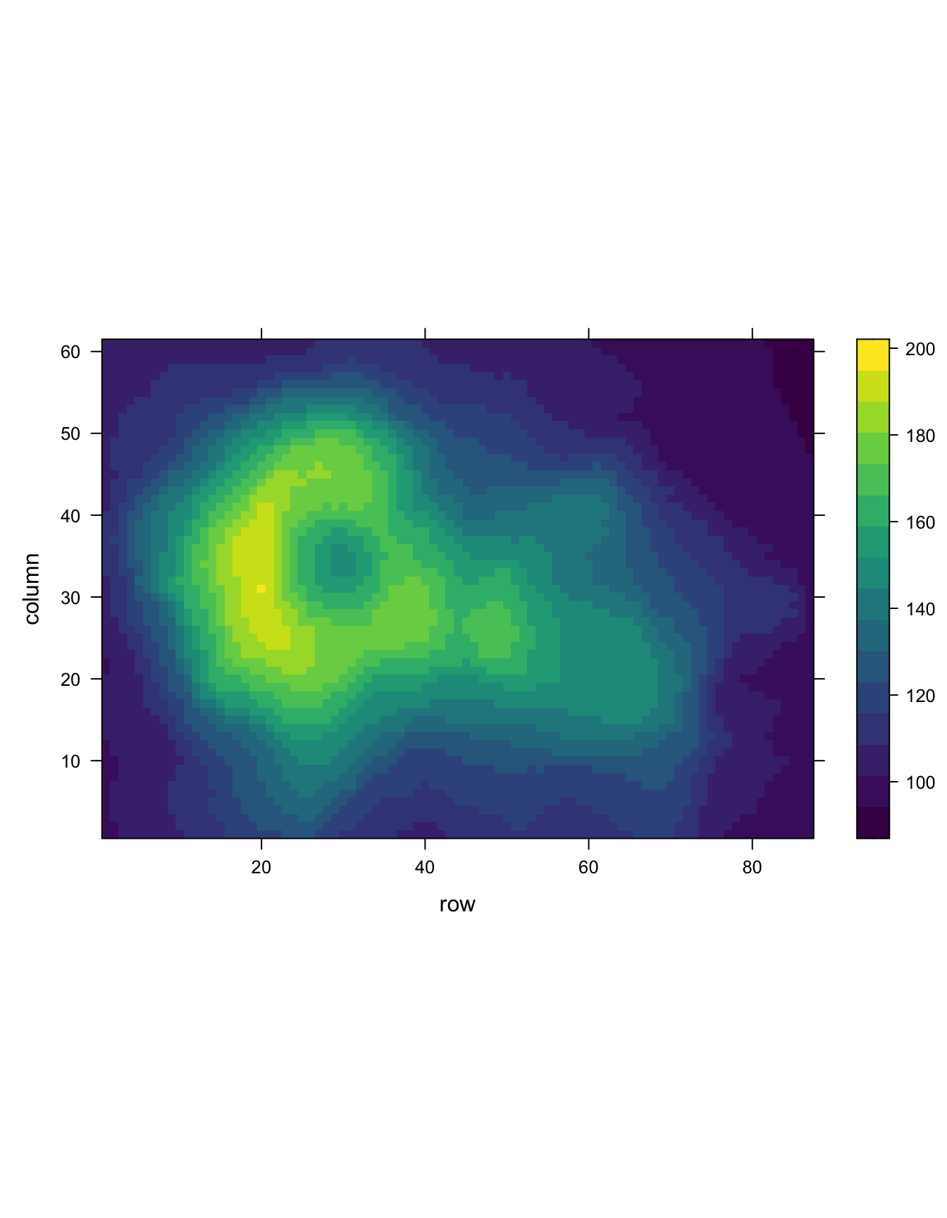
# 3: Viridis
library(viridisLite)
coul <- viridis(100)
levelplot(volcano, col.regions = coul) 
#levelplot(volcano, col.regions = magma(100))

Heatmap with lattice and levelplot()

Basis use of levelplot()

From wide input matrix

Flip and reorder axis

Custom colors

❤️ 10 best R tricks ❤️