Most basic Heatmap
How to do it: below is the most basic
heatmap you can build in base R, using
the heatmap() function with no parameters. Note that
it takes as input a matrix. If you have a data frame, you can
convert it to a matrix with as.matrix(), but you need
numeric variables only.
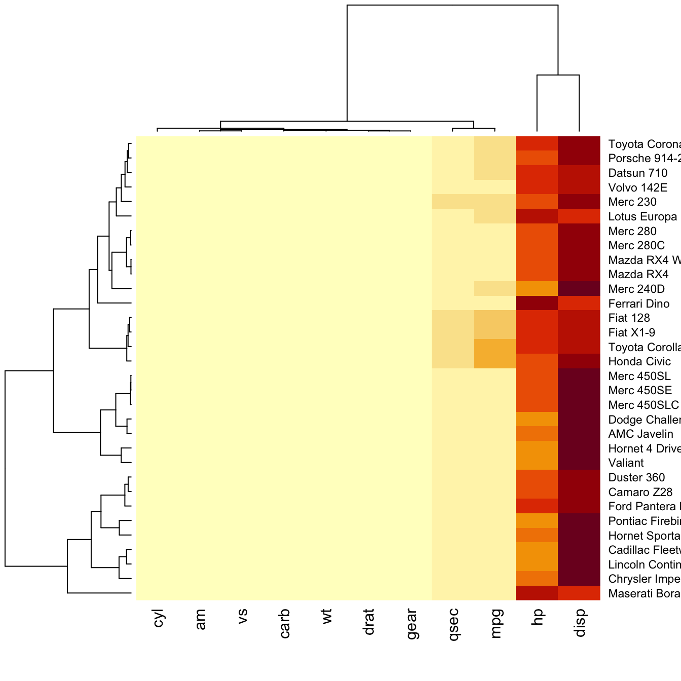
How to read it: each column is a variable. Each observation
is a row. Each square is a value, the closer to yellow the higher.
You can transpose the matrix with t(data) to swap X
and Y axis.
Note: as you can see this heatmap is not very insightful:
all the variation is absorbed by the hp and
disp variables that have very high values compared to
the others. We need to normalize the data, as explained in the
next section.
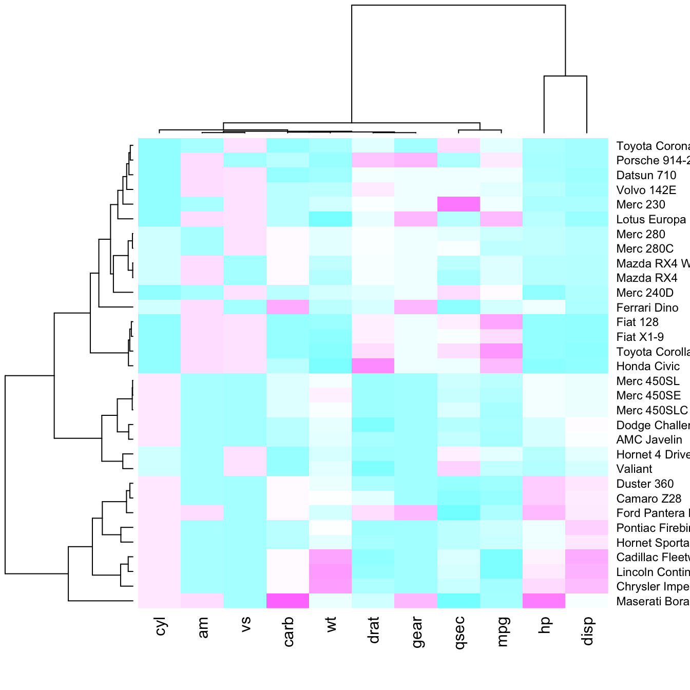
Normalization
Normalizing the matrix is done using the
scale argument of the
heatmap() function. It can be applied to
row or to column. Here the
column option is chosen, since we need to absorb the
variation between column.
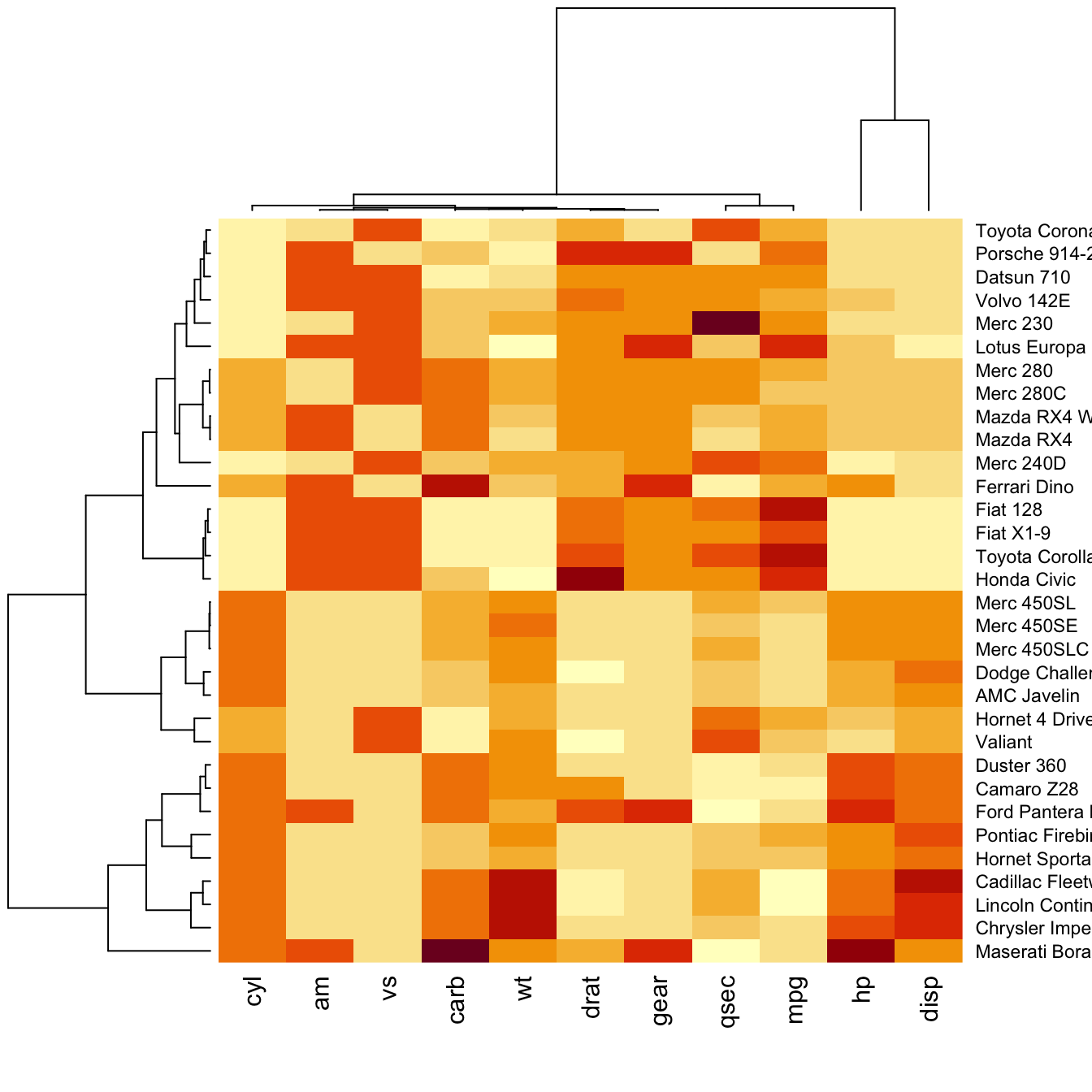
Dendrogram and Reordering
You may have noticed that order of both rows and columns is
different compare to the native mtcar matrix. This is
because heatmap() reorders both variables and
observations using a clustering algorithm: it computes the
distance between each pair of rows and columns and try to order
them by similarity.
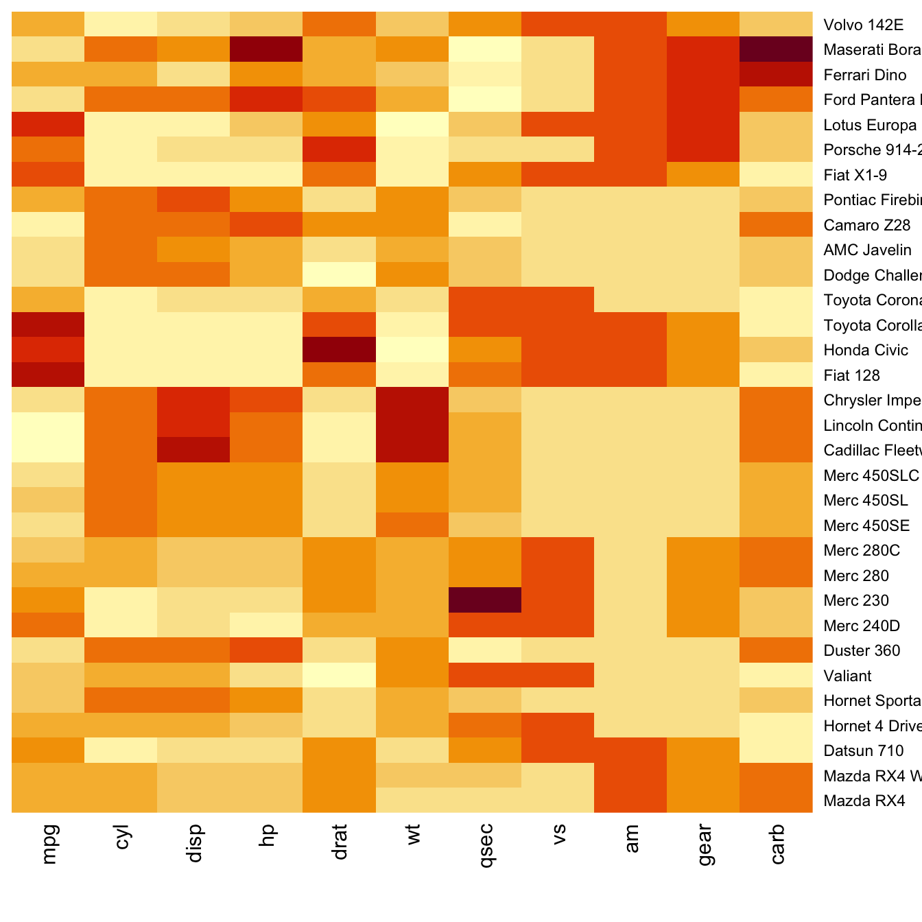
Moreover, the corresponding dendrograms are provided
beside the heatmap. We can avoid it and just visualize the raw
matrix: use the Rowv and Colv arguments
as follow.
Color palette
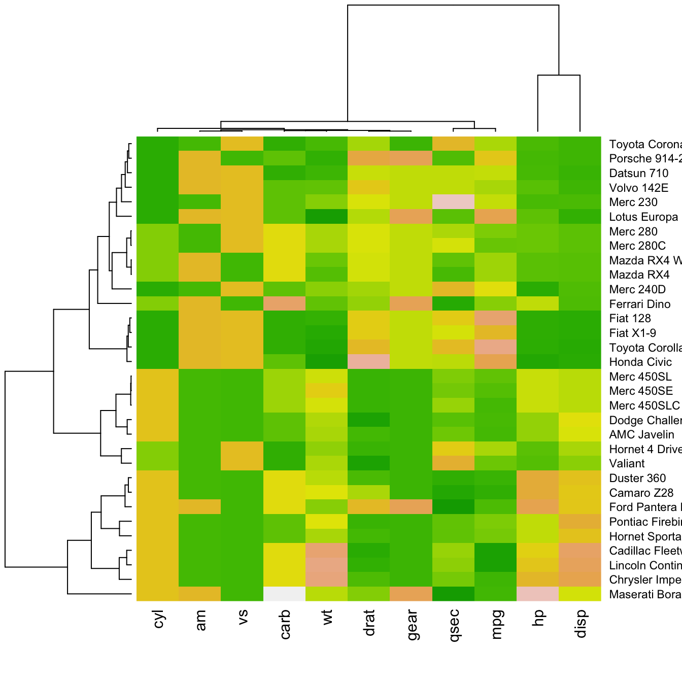
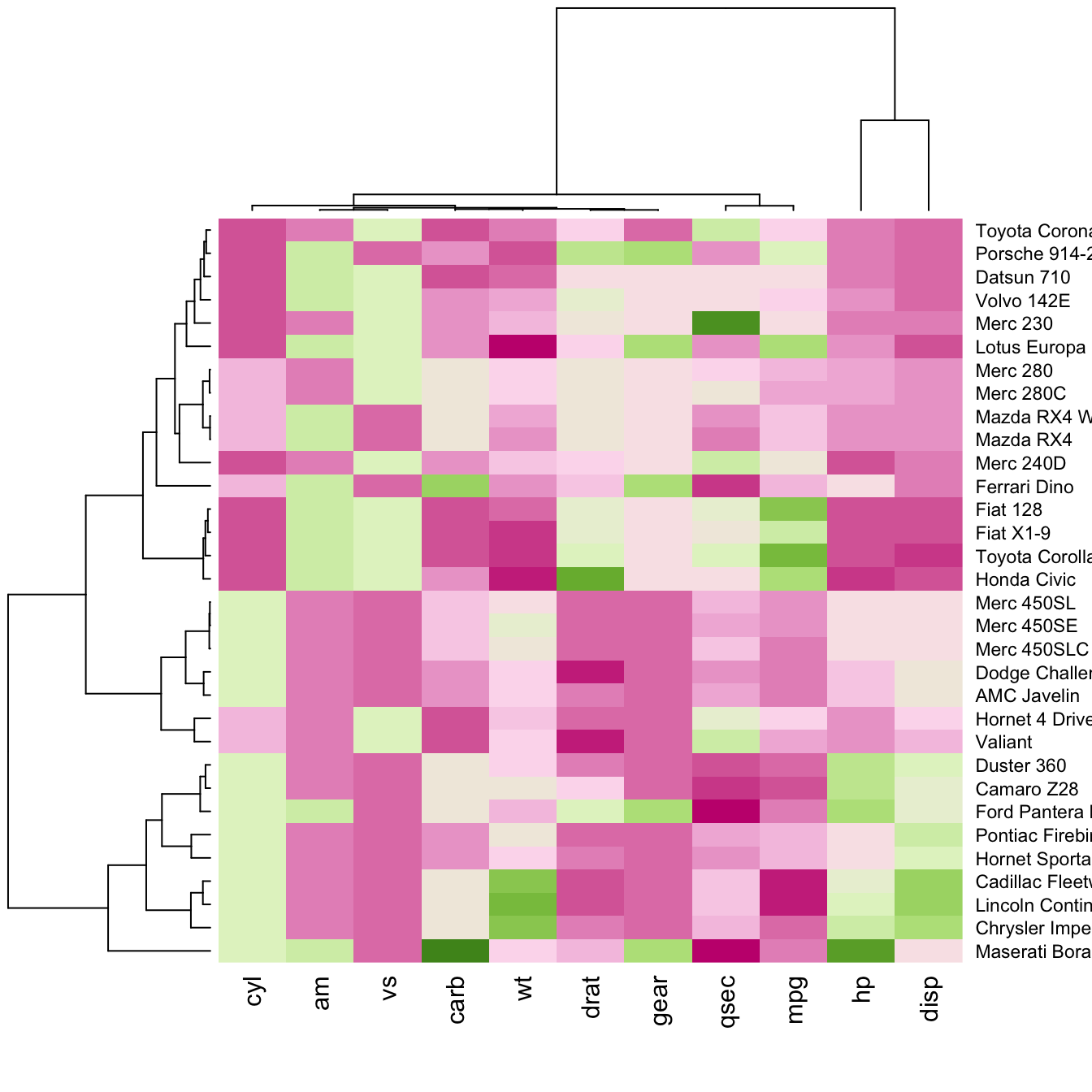
There are several ways to custom the color palette:
-
use the native palettes of R:
terrain.color(),rainbow(),heat.colors(),topo.colors()orcm.colors() -
use the palettes proposed by
RColorBrewer. See list of available palettes here.
Custom Layout
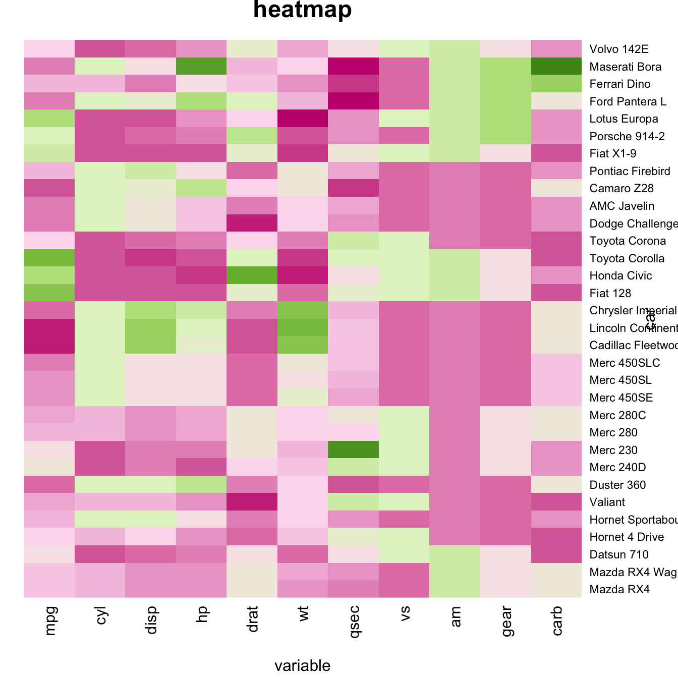
You can custom title & axis titles with the usual
main and xlab/ylab arguments
(left).
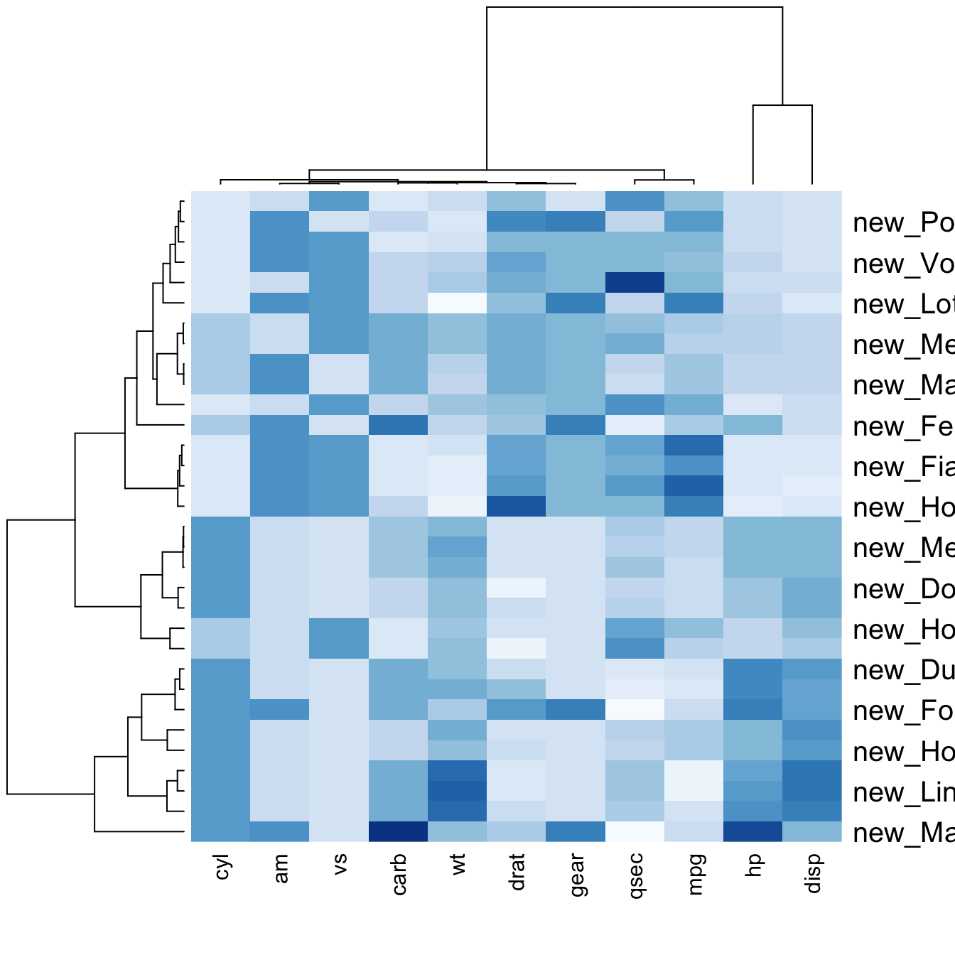
You can also change labels with labRow/colRow
and their size with cexRow/cexCol.
# Add classic arguments like main title and axis title
heatmap(data, Colv = NA, Rowv = NA, scale="column", col = coul, xlab="variable", ylab="car", main="heatmap")
# Custom x and y labels with cexRow and labRow (col respectively)
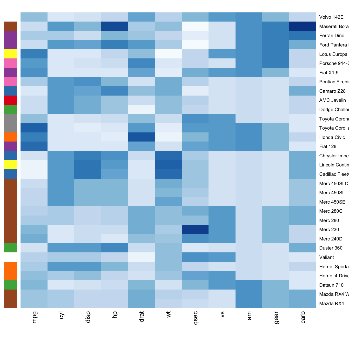
heatmap(data, scale="column", cexRow=1.5, labRow=paste("new_", rownames(data),sep=""), col= colorRampPalette(brewer.pal(8, "Blues"))(25))Add color beside heatmap
Often, heatmap intends to compare the observed structure with an expected one.
You can add a vector of color beside the heatmap to represents the
expected structure using the RowSideColors argument.