Create summary and presentation ready tables with gtsummary


This post explains how to use the 
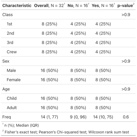
gtsummary package for creating table summary, especially with descriptive statistics, regression models, medical values or demographics data.
This post showcases the key features of gtsummary and provides a set of table examples using the package.

Documentation

{gtsummary}

Quick start


The gtsummary package in R is made for creating tables that summarize information, statistics or more in a given dataset. You can use it in combination of the pipe %>% symbol for easy-to-read code and publication-ready tables!

The main function is tbl_summary() that becomes very powerful when combined with other functions available. If you’re working a regression problem, you have the tbl_regression() function. If you need to merge some tables, you have tbl_merge(). Those are just examples of things you can do!

✍️ author → Daniel D. Sjoberg

📘 documentationgithub

⭐️ more than 800 stars on github

Characteristic Drug, N = 571 Placebo, N = 431 Difference2 95% CI2,3 p-value2
age

-0.57 -4.4, 3.2 0.8
    Median (IQR) 51 (45, 56) 51 (45, 59)


sex

0.17 -0.23, 0.57
    Female 30 (53%) 19 (44%)


    Male 27 (47%) 24 (56%)


bmi

0.75 -1.1, 2.6 0.4
    Median (IQR) 25.3 (21.9, 28.8) 23.6 (21.4, 26.3)


1 n (%)
2 Welch Two Sample t-test; Standardized Mean Difference
3 CI = Confidence Interval

Installation


To get started with gtsummary, you can install it directly from CRAN using the install.packages function:

install.packages("gtsummary")

Basic usage


The gtsummary package lets you automatically summarize information about your dataset. In the following case, we use the tbl_summary() function to obtain the main information on the iris dataset. The package detects the variable type and generates the appropriate summary type.

data(iris)
library(gtsummary)

iris %>%
  tbl_summary()
Characteristic N = 1501
Sepal.Length 5.80 (5.10, 6.40)
Sepal.Width 3.00 (2.80, 3.30)
Petal.Length 4.35 (1.60, 5.10)
Petal.Width 1.30 (0.30, 1.80)
Species
    setosa 50 (33%)
    versicolor 50 (33%)
    virginica 50 (33%)
1 Median (IQR); n (%)

Key features


→ Regression model results

With the tbl_regression() function, we can super easily display the statistical results of a regression model.

Example with a logistic regression on the Titanic dataset:

# load dataset
data(Titanic)
df = as.data.frame(Titanic)

# load library
library(gtsummary)

# create the model
model = glm(Survived ~ Age + Class + Sex + Freq, family=binomial, data=df)

# generate table 
model %>%
  tbl_regression() %>% # regression summary function
  add_global_p() %>% # add p-values
  bold_labels() %>% # make label in bold
  italicize_levels() # make categories in label in italic
Characteristic log(OR)1 95% CI1 p-value
Age

0.5
    Child
    Adult 0.62 -1.0, 2.4
Class

>0.9
    1st
    2nd -0.03 -2.0, 2.0
    3rd 0.25 -1.8, 2.4
    Crew 0.27 -1.8, 2.4
Sex

0.6
    Male
    Female -0.37 -1.9, 1.1
Freq -0.01 -0.02, 0.00 0.2
1 OR = Odds Ratio, CI = Confidence Interval

→ Summarize table

As its name suggests it, the gtsummary package makes very easy to generate summary of your dataset. In practice, it uses the tbl_summary() function to compute descriptive statistics for every column in your dataset depending to the type of variable.

What’s even better is that you can add inferential statistics (like p-values) to these tables to make them even more informative!

Example:

# load dataset and filter to keep just a few columns
data(mtcars) 
mtcars = mtcars %>%
  select(vs, mpg, drat, hp, gear)

# load package
library(gtsummary)

# create summary table
mtcars %>%
  tbl_summary(
    by=vs, # group by the `vs` variable (dichotomous: 0 or 1)
    statistic = list(
      all_continuous() ~ "{mean} ({sd})", # will display: mean (standard deviation)
      all_categorical() ~ "{n} / {N} ({p}%)" # will display: n / N (percentage)
    )
  ) %>%
  add_overall() %>% # statistics for all observations
  add_p() %>% # add p-values
  bold_labels() %>% # make label in bold
  italicize_levels() # make categories in label in italic
Characteristic Overall, N = 321 0, N = 181 1, N = 141 p-value2
mpg 20.1 (6.0) 16.6 (3.9) 24.6 (5.4) <0.001
drat 3.60 (0.53) 3.39 (0.47) 3.86 (0.51) 0.013
hp 147 (69) 190 (60) 91 (24) <0.001
gear


0.001
    3 15 / 32 (47%) 12 / 18 (67%) 3 / 14 (21%)
    4 12 / 32 (38%) 2 / 18 (11%) 10 / 14 (71%)
    5 5 / 32 (16%) 4 / 18 (22%) 1 / 14 (7.1%)
1 Mean (SD); n / N (%)
2 Wilcoxon rank sum test; Fisher’s exact test

→ Custom style of the table

The package has a whole set of functions that can be used to custom what your table looks like. You can even call functions from others packages such as gt

Example:

data(iris)
library(gtsummary)
library(gt)

iris %>%
  tbl_summary(by=Species) %>%
  add_overall() %>% # info ignoring the `by` argument
  add_n() %>% # number of observations
  modify_header(label ~ "**Variables from the dataset**") %>% # title of the variables
  modify_spanning_header(c("stat_0", "stat_1", "stat_2", "stat_3") ~ "*Descriptive statistics of the iris flowers*, grouped by Species") %>%
  as_gt() %>%
  gt::tab_source_note(gt::md("*The iris dataset is probably the **most famous** dataset in the world*"))
Variables from the dataset N Descriptive statistics of the iris flowers, grouped by Species
Overall, N = 1501 setosa, N = 501 versicolor, N = 501 virginica, N = 501
Sepal.Length 150 5.80 (5.10, 6.40) 5.00 (4.80, 5.20) 5.90 (5.60, 6.30) 6.50 (6.23, 6.90)
Sepal.Width 150 3.00 (2.80, 3.30) 3.40 (3.20, 3.68) 2.80 (2.53, 3.00) 3.00 (2.80, 3.18)
Petal.Length 150 4.35 (1.60, 5.10) 1.50 (1.40, 1.58) 4.35 (4.00, 4.60) 5.55 (5.10, 5.88)
Petal.Width 150 1.30 (0.30, 1.80) 0.20 (0.20, 0.30) 1.30 (1.20, 1.50) 2.00 (1.80, 2.30)
The iris dataset is probably the most famous dataset in the world
1 Median (IQR)


Contact

This document is a work by Yan Holtz. Any feedback is highly encouraged. You can fill an issue on Github, drop me a message on Twitter, or send an email pasting yan.holtz.data with gmail.com.

Github Twitter