The tmap package in R is
designed for creating thematic maps, allowing users to
visualize spatial data in an intuitive and flexible way.
This post
showcases the key features of tmap and
provides a set of map examples using the package.
{tmap}
The tmap package in R is designed for creating
thematic maps, allowing users to visualize spatial data
in an intuitive and flexible way.
To get started with tmap, you can install it directly
from CRAN using the install.packages function:
The tmap package uses a layered approach to building
maps, similar to ggplot2. You
start with tm_shape() to define the data, then add layers
with various tm_*() functions.
Here’s a basic example:
library(tmap)
data("World")
tm_shape(World) +
tm_polygons("pop_est", style = "quantile", title = "Population")
You can create minimalist maps using the
tm_borders() function:

You can add multiple layers to your map using the
+ operator. The following example will add the
name of each country with a size proportional
to the AREA column:
library(tmap)
data("World")
tm_shape(World) +
tm_polygons("income_grp", palette = "Blues") +
tm_text("name", size = "AREA")
Use tm_facets() to create small multiples based
on a variable. Here, we use the continent column
to create a facet:
library(tmap)
data("World")
tm_shape(World) +
tm_polygons("gdp_cap_est", style = "quantile") +
tm_facets("continent", free.coords = FALSE)
You can apply any custom style to your tmap maps. In the
following example, we:
library(tmap)
library(dplyr)
# Prepare the data
data("World")
world_data <- World %>%
filter(!is.na(life_exp)) %>%
mutate(pop_density = pop_est / area)
# Create the customized map
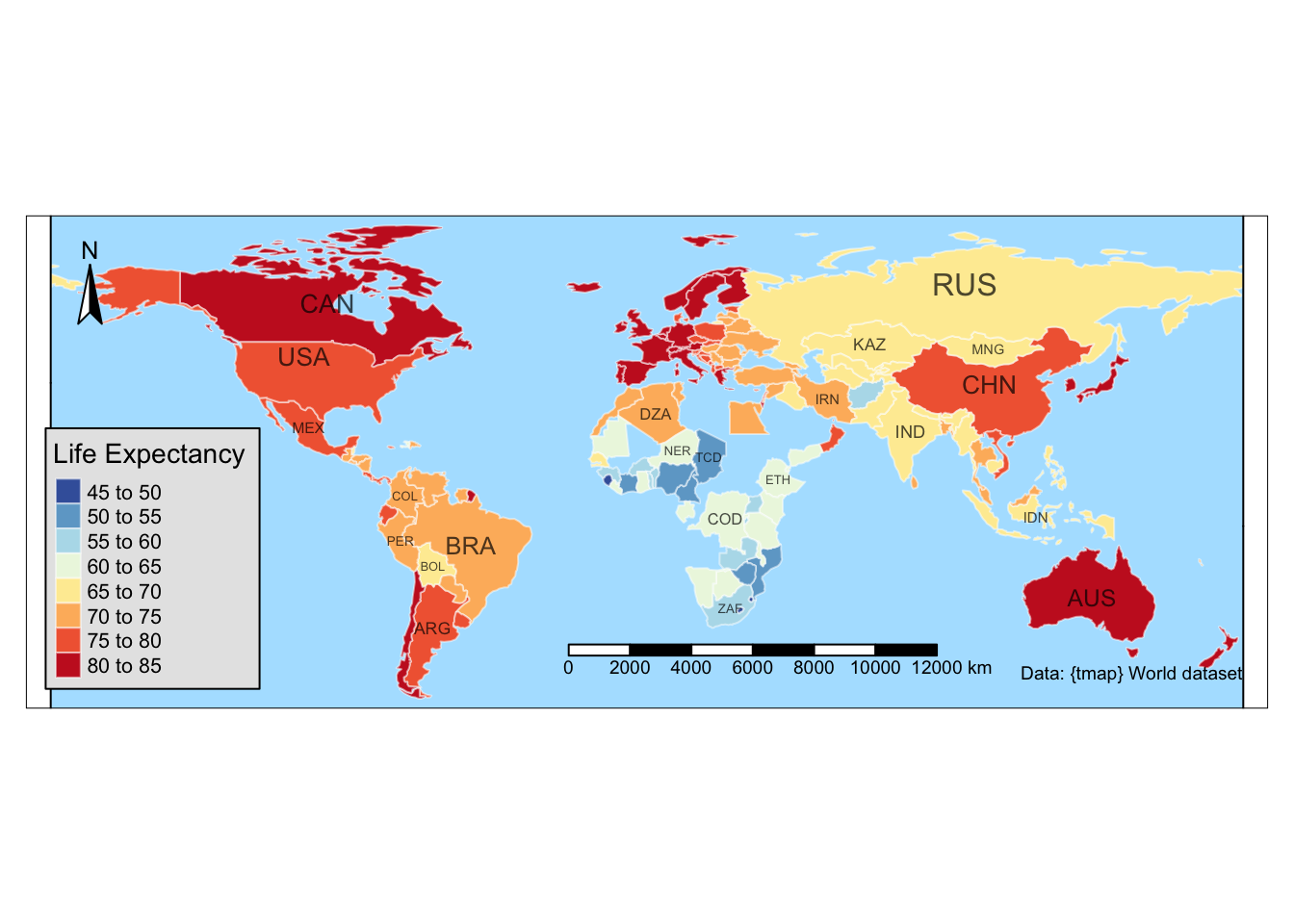
tm_shape(world_data) +
tm_polygons("life_exp",
palette = "-RdYlBu",
style = "pretty",
n = 7,
title = "Life Expectancy",
popup.vars = c("name", "life_exp", "gdp_cap_est"),
border.col = "white",
border.alpha = 0.5
) +
tm_text("iso_a3", size = "AREA", col = "black", fontface = "bold", alpha = 0.7) +
tm_layout(
title = "Global Life Expectancy and Economic Indicators",
title.position = c("center", "top"),
title.size = 1.5,
bg.color = "#f5f5f5",
inner.margins = c(0.1, 0.1, 0.1, 0.1),
frame = TRUE,
frame.lwd = 2,
legend.outside = TRUE,
legend.outside.position = "right",
legend.frame = TRUE,
legend.bg.color = "white",
legend.text.size = 0.7
) +
tm_compass(position = c("left", "top"), size = 2) +
tm_scale_bar(position = c("left", "bottom"), text.size = 0.6) +
tm_credits("Data: {tmap} World dataset", position = c("right", "bottom"), size = 0.6) +
tm_style("natural")
You can super easily make all your tmap maps switch to
interactive mode with tmap_mode("view"). In this example,
we:
library(tmap)
library(dplyr)
data("World")
europe <- World %>%
filter(continent == "Europe")
tmap_mode("view")
my_tmap <- tm_shape(europe) +
tm_polygons("gdp_cap_est",
style = "jenks",
palette = "viridis",
title = "GDP per capita",
popup.vars = c("name", "pop_est", "gdp_cap_est"),
id = "name"
) +
tm_borders(alpha = 0.5) +
tm_bubbles(
size = "pop_est",
col = "life_exp",
scale = 0.5,
title.size = "Population",
title.col = "Life Expectancy",
popup.vars = TRUE
) +
tm_layout(
title = "European Countries: GDP, Population, and Life Expectancy",
legend.outside = TRUE,
legend.outside.position = "right"
) +
tm_scale_bar(position = c("left", "bottom")) +
tm_compass(position = c("right", "top"))
tmap_save(my_tmap, filename = "../HtmlWidget/my_interactive_map.html")Note: You can return to static display mode by
running:tmap_mode("plot")
If you want to learn more about tmap, it’s highly
suggested to have a look at:
👋 After crafting hundreds of R charts over 12 years, I've distilled my top 10 tips and tricks. Receive them via email! One insight per day for the next 10 days! 🔥