Quick start

The paletteer package in R brings together all the color palettes from a large number of R packages dedicated to colours. It provides a simple and consistent interface to access these palettes, making it easy to work with any color palette in R.

It offers more than 2000 color palettes from various R packages, making it easy to create beautiful and informative visualizations.

✍️ author → Emil Hvitfeldt

📘 documentation → github

⭐️ more than 800 stars on github

Installation

To get started with paletteer, you can install it directly from CRAN using the install.packages function:

install.packages("paletteer")

Basic usage

If you want to easily get started with paletteer, you can use the paletteer_d() function to access the palettes.

paletteer has a straightforward syntax for accessing palettes: package_name::palette_name.

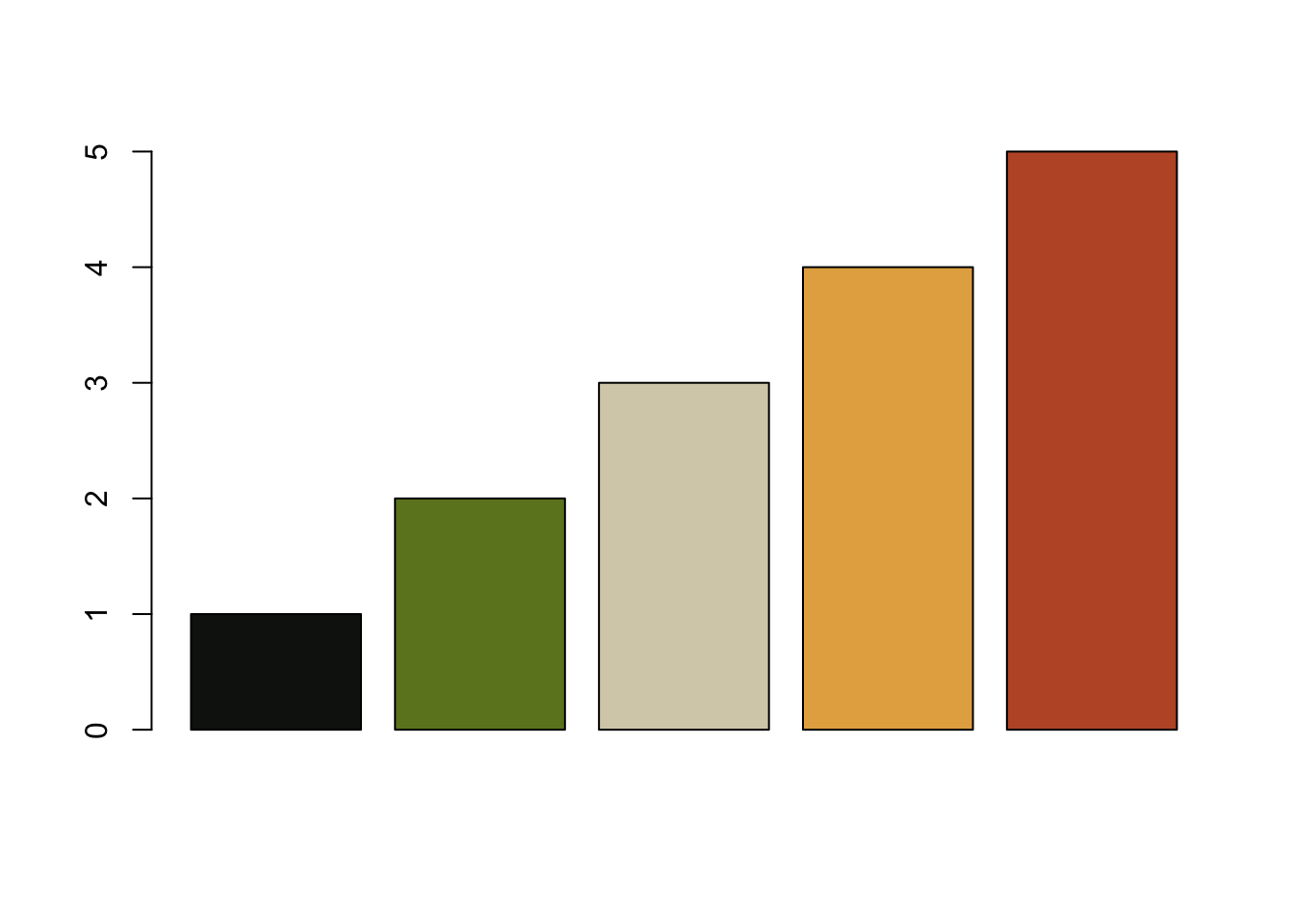
Here’s a basic example with the FridaKahlo palette from the lisa package:

# load the library
library(paletteer)

# get the palette
my_colors <- paletteer::paletteer_d("lisa::FridaKahlo")

# use colors in a plot
barplot(1:length(my_colors), col = my_colors)

Key features

Palettes have different types, and paletteer demands a specific function to access each type.

For example, if you want to build a choropleth map, you need a continuous palette. In this case, you can use the paletteer_s and scale_fill_paletteer_c functions.

For a bar plot, you need a discrete palette. In this case, you can use the paletteer_d and scale_fill_paletteer_d functions.

→ Diverging continuous palettes

A diverging continuous palette is a palette that has a center and two extremes. It is useful for visualizing data with a center value.

For example, a palette that goes from blue to white to red is a diverging continuous palette.

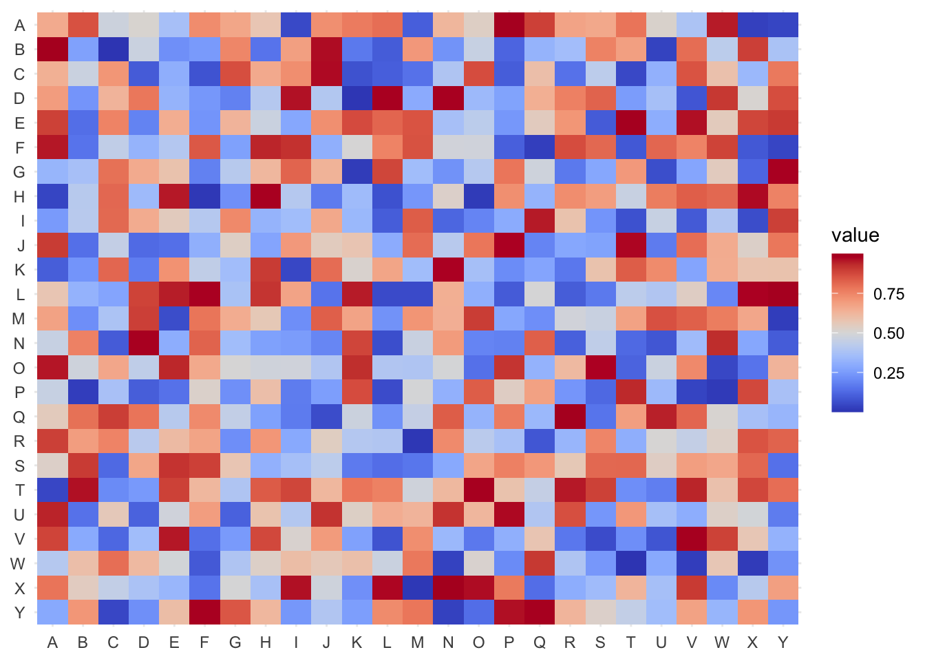
Example with the pals::coolwarm palette:

# load required libraries
library(ggplot2)
library(paletteer)
library(reshape2)

# create a sample matrix to simulate data
set.seed(123)
data_matrix <- matrix(runif(625, min = 0, max = 1), nrow = 25, ncol = 25)
rownames(data_matrix) <- rev(LETTERS[1:25])
colnames(data_matrix) <- LETTERS[1:25]
data <- melt(data_matrix)

# create the heatmap
ggplot(data, aes(x = Var2, y = Var1, fill = value)) +
  geom_tile() +
  scale_fill_paletteer_c("pals::coolwarm") +
  labs(x = NULL, y = NULL) +
  theme_minimal()

→ Sequential continuous palettes

A sequential continuous palette is a palette that goes from one extreme to another. It is useful for visualizing data that goes from low to high.

For example, a palette that goes from purple to light yellow is a sequential continuous palette.

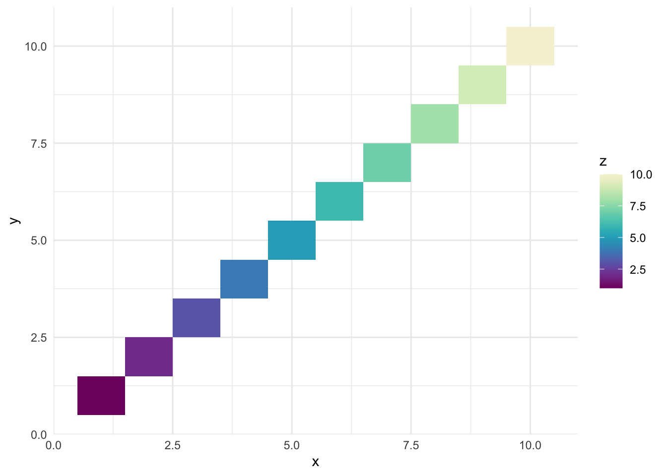
Example with grDevices::Purple-Yellow palette:

# load the library
library(paletteer)
library(ggplot2)

# create some data
data <- data.frame(x = 1:10, y = 1:10, z = 1:10)

# create a plot
ggplot(data, aes(x, y, fill = z)) +
  geom_tile() +
  scale_fill_paletteer_c("grDevices::Purple-Yellow") +
  theme_minimal()

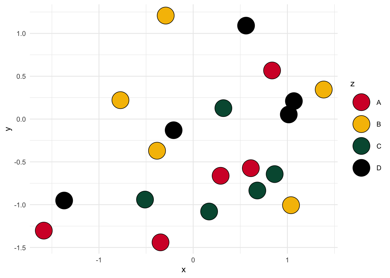
→ Qualitative discrete palettes

Discrete palettes are palettes that have a fixed number of colors. They are useful for visualizing data that is categorical.

For example, a palette that goes from red to orange to green to black is a discrete palette.

Example with the nbapalettes::supersonics_holiday palette:

# load the library
library(paletteer)
library(ggplot2)

# create some data
data <- data.frame(
  x = rnorm(20),
  y = rnorm(20),
  z = rep(LETTERS[1:4], 5)
)

# create a plot
ggplot(data, aes(x, y, fill = z)) +
  geom_point(size = 10, shape = 21) +
  scale_fill_paletteer_d("nbapalettes::supersonics_holiday") +
  theme_minimal()

→ Get colors from a palette

Since discrete palettes contains a fixed number of colors, you can also use paletteer to retrieve a list of colors and not just using them in a plot.

Example:

# load the library
library(paletteer)

# get the palette
my_colors <- paletteer::paletteer_d("lisa::FridaKahlo")
print(my_colors)

## <colors>
## #121510FF #6D8325FF #D6CFB7FF #E5AD4FFF #BD5630FF

Gallery of paletteer examples

The gallery has a dedicated page to showcase all available palettes in paletteer with reproducible code and examples. Browse them to find your dream palette!

Use any color palette with paletteer