Stacked area with ggplot2
The data frame used as input to build a stacked area chart requires 3 columns:
-
x: numeric variable used for the X axis, often it is a time. -
y: numeric variable used for the Y axis. What are we looking at? group: one shape will be done per group.
The chart is built using the geom_area() function.
# Packages
library(ggplot2)
library(dplyr)
# create data
time <- as.numeric(rep(seq(1,7),each=7)) # x Axis
value <- runif(49, 10, 100) # y Axis
group <- rep(LETTERS[1:7],times=7) # group, one shape per group
data <- data.frame(time, value, group)
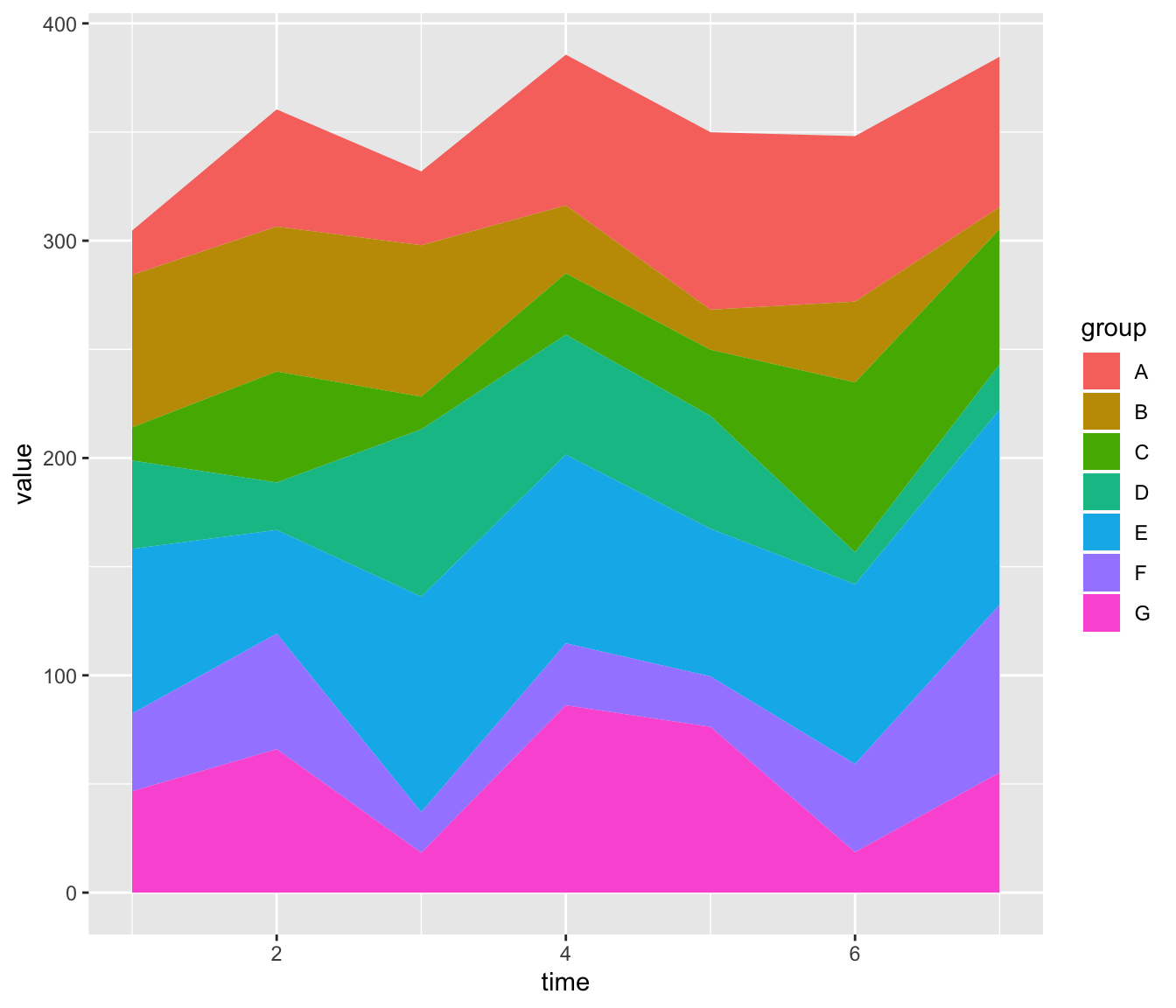
# stacked area chart
ggplot(data, aes(x=time, y=value, fill=group)) +
geom_area()Control stacking order with ggplot2
The gallery offers a post dedicated to reordering with ggplot2. This step can be tricky but the code below shows how to:
-
give a specific order with the
factor()function. - order alphabetically using
sort() - order following values at a specific data
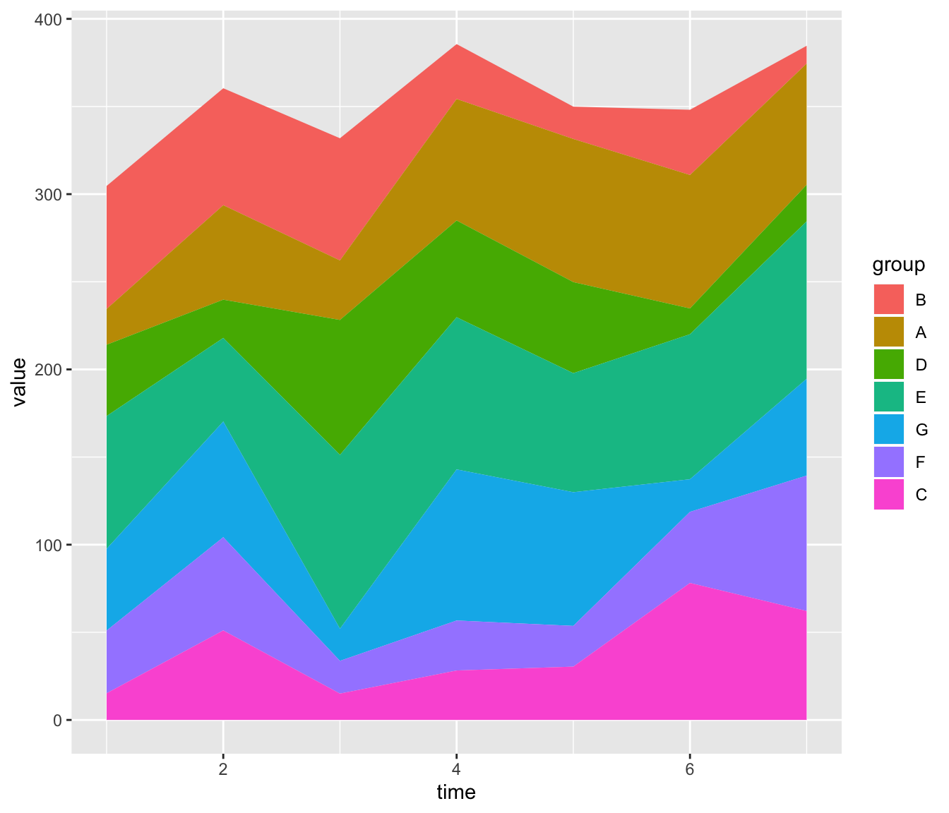
# Give a specific order:
data$group <- factor(data$group , levels=c("B", "A", "D", "E", "G", "F", "C") )
# Plot again
ggplot(data, aes(x=time, y=value, fill=group)) +
geom_area()
# Note: you can also sort levels alphabetically:
myLevels <- levels(data$group)
data$group <- factor(data$group , levels=sort(myLevels) )
# Note: sort following values at time = 5
myLevels <- data %>%
filter(time==6) %>%
arrange(value)
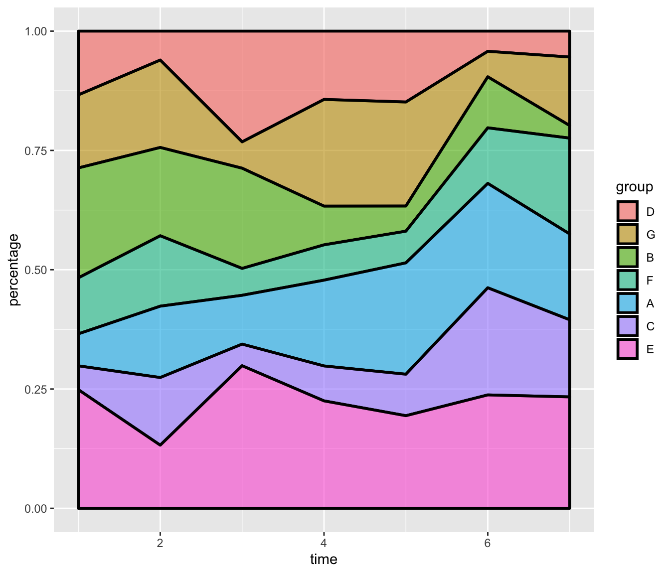
data$group <- factor(data$group , levels=myLevels$group )Proportional stacked area chart
In a proportional stacked area graph, the sum of each year is always equal to hundred and value of each group is represented through percentages.
To make it, you have to calculate these percentages first. This
can be done using dplyr of with base R.
# Compute percentages with dplyr
library(dplyr)
data <- data  %>%
  group_by(time, group) %>%
  summarise(n = sum(value)) %>%
  mutate(percentage = n / sum(n))

# Plot
ggplot(data, aes(x=time, y=percentage, fill=group)) +
    geom_area(alpha=0.6 , size=1, colour="black")

# Note: compute percentages without dplyr:
my_fun <- function(vec){
  as.numeric(vec[2]) / sum(data$value[data$time==vec[1]]) *100
}
data$percentage <- apply(data , 1 , my_fun)
Color & style
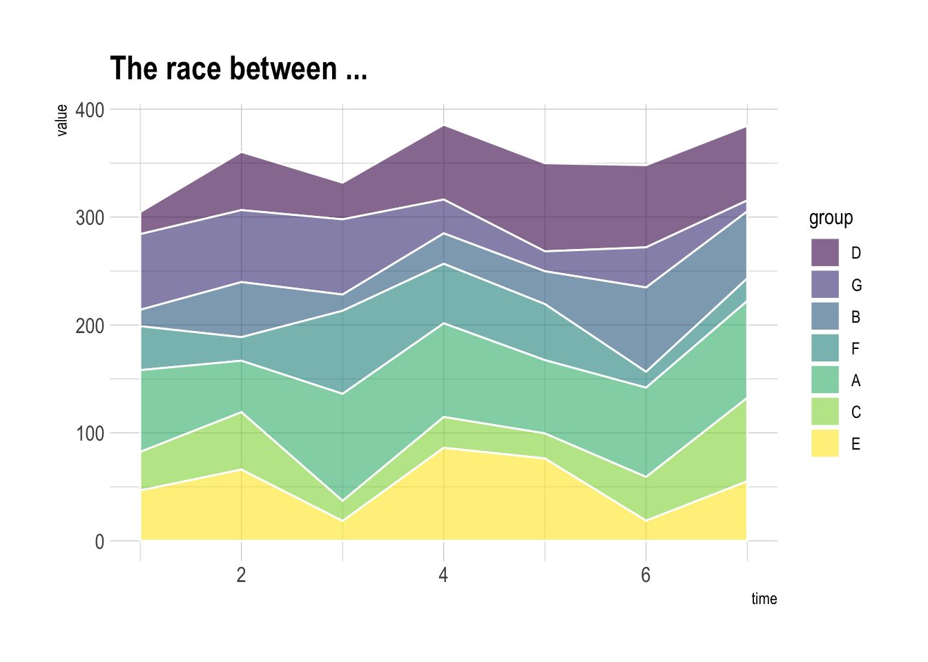
Let’s improve the chart general appearance:
- usage of the
viridiscolor scale -
theme_ipsumof thehrbrthemespackage - add title with
ggtitle
# Library
library(viridis)
library(hrbrthemes)

# Plot
ggplot(data, aes(x=time, y=value, fill=group)) +
    geom_area(alpha=0.6 , size=.5, colour="white") +
    scale_fill_viridis(discrete = T) +
    theme_ipsum() +
    ggtitle("The race between ...")