If you did not find the geospatial data you need in existing R packages (see the map section), you need to find this information elsewhere on the web.
It will often be stored as a .geoJSON format. This post
explains how to read it.
Find and download a .geoJSON file
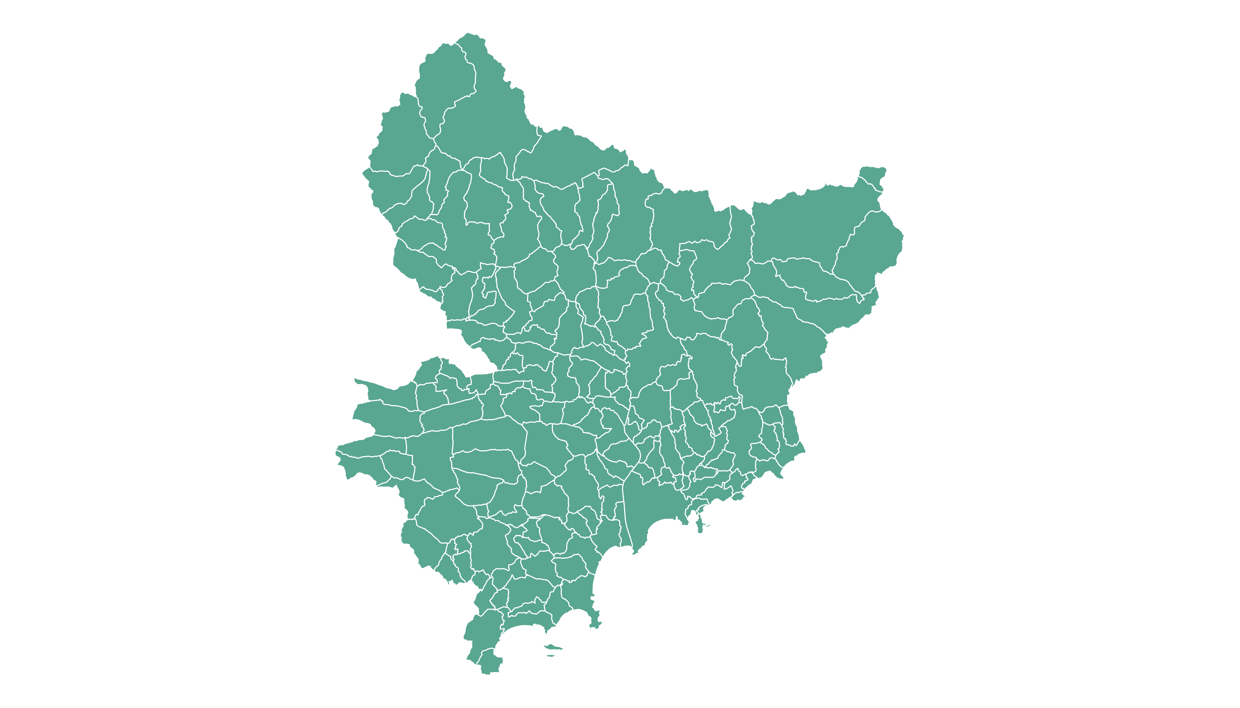
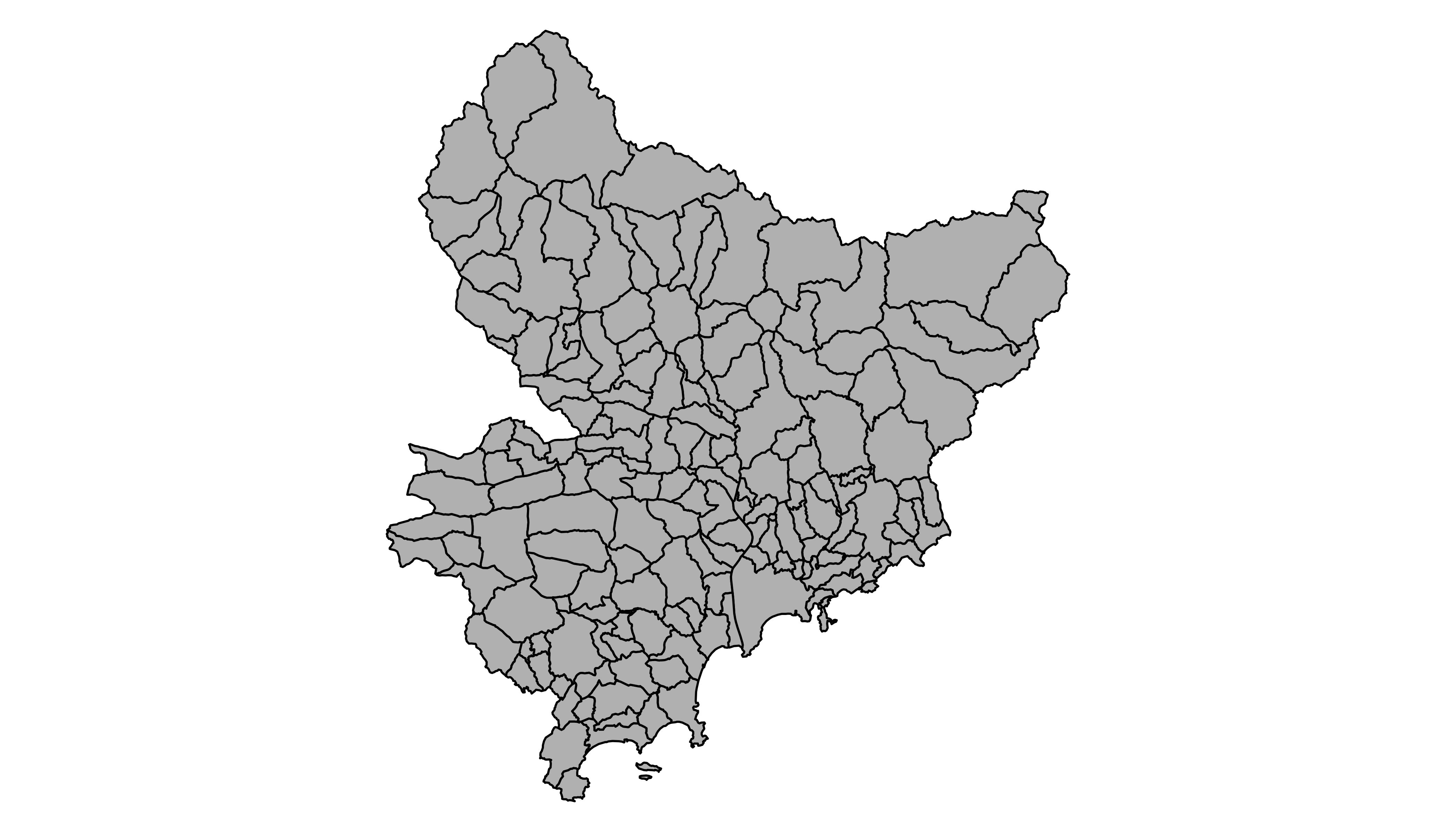
You need to dig the internet to find the geoJSON file you are interested in. For instance, this URL provides a file containing french region boundaries.
You can load it in R with:
# Download to a temporary file
tmp_geojson <- tempfile(fileext = ".geojson")
download.file(
  "https://raw.githubusercontent.com/gregoiredavid/france-geojson/master/communes.geojson",
  tmp_geojson
)

# Let's read the downloaded geoJson file with the sf library:
library(sf)
my_sf <- read_sf(tmp_geojson)
That’s it! You now have a geospatial object called my_sf.
I strongly advise to read
this post to
learn how to manipulate it.
Just in case, here is how to plot it in base R and with
ggplot2.
Plot it with base R
The basic plot() function knows how to plot a
geospatial object. Thus you just need to pass it
my_sf and add a couple of options to customize the
output.
Plot it with ggplot2
It is totally possible (and advised IMO) to build the map with
ggplot2, using the
geom_sf() function as described below.