Libraries
The rayshader package makes it simple to create shaded 2D relief maps.
Since the package is on CRAN, you can
install it with
install.packages("rayshader").
We also load the raster package to
access data to work with.
Data format
The rayshader package requires input data in an elevation matrix format. This is a specific matrix where each cell holds the elevation value for the corresponding map point.
Here’s how to obtain the elevation matrix of the
Grand Canyon from a raster file using the
raster package.
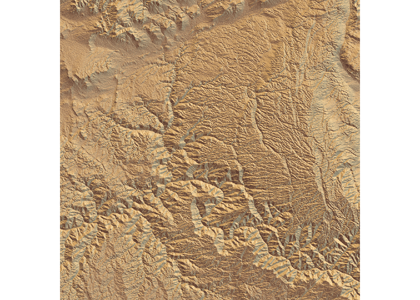
Basic 2D map
Let’s see how to create a basic 2D map with rayshader.
We use the sphere_shade() function to create the map. It
takes the elevation matrix as input and returns a
shaded map, and then plot it with the
plot_map() function.
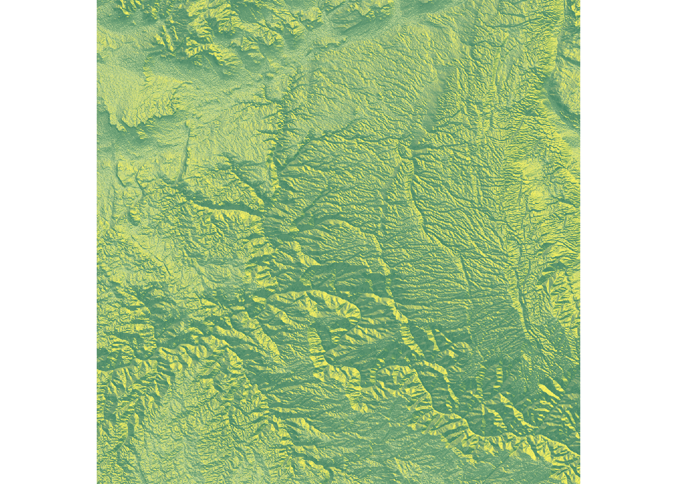
Change texture
rayshader includes a
specialized function to create textures:
create_texture(). This function accepts
5 colors as input and generates a texture suitable
for use in the sphere_shade() function.
custom_texture <- create_texture("#fff673","#55967a","#8fb28a","#55967a","#cfe0a9")

elevation_matrix %>%
  sphere_shade(texture=custom_texture, sunangle = 45) %>%
  plot_map()
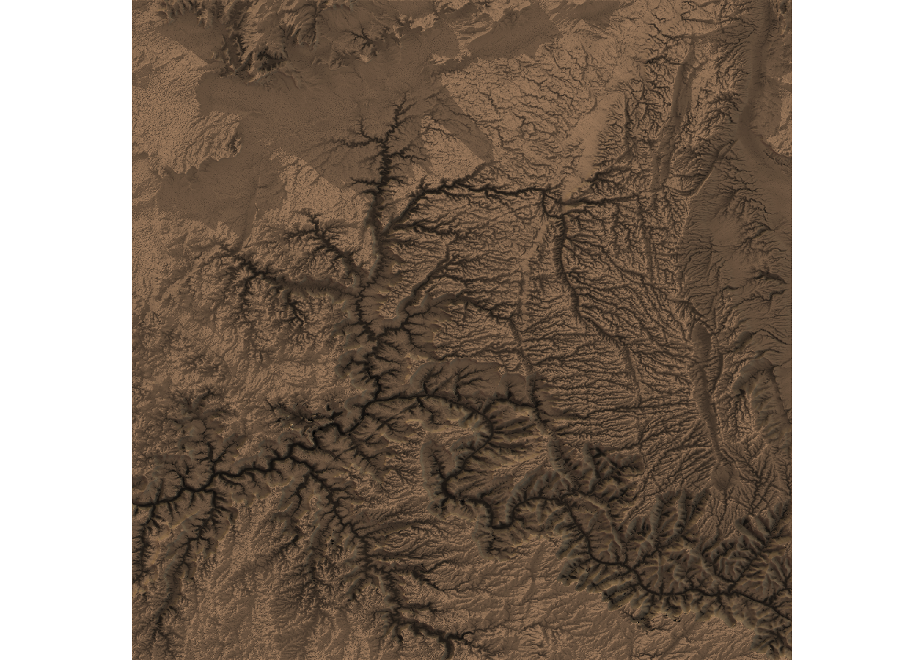
Change shade properties
The add_shadow() function can be used to add a shadow to
the map. The ray_shade() function creates a shadow based
on the sun angle, while the ambient_shade() function
creates a shadow based on the ambient light.
elevation_matrix %>%
  sphere_shade(texture="desert", sunangle = 45, zscale = 50) %>%
  add_shadow(ray_shade(elevation_matrix), 0.5) %>%  # Adds a ray-traced shadow
  add_shadow(ambient_shade(elevation_matrix), 0) %>%  # Adds an ambient shadow
  plot_map()
Going further
You might be interested in
- creating 3d maps with rayshader
- learning more about rayshader